Thursday 31 March 2016

The Book is Out!

Finally, the book is out!

Make Your Own Neural Network - a gentle introduction to the mathematics of neural networks, and making your own with Python.


You can get it on Amazon Kindle, and a paper print version is also be available.

Sunday 13 March 2016

IPython Neural Networks on a Raspberry Pi Zero

There is an updated version of this guide at http://makeyourownneuralnetwork.blogspot.co.uk/2017/01/neural-networks-on-raspberry-pi-zero.html


In this post we will aim to get IPython set up on a Raspberry Pi.


There are several reasons for doing this:

  • Raspberry Pis are fairly cheap and accessible to many more people than expensive laptops.
  • Raspberry Pis are very open - they run the free and open source Linux operating system, together with lots of free and open source software, including Python. Open source is important because it is important to understand how things work, to be able to share your work and enable others to build on your work. Education should be about learning how things work, and making your own, and not be about learning to buy closed proprietary software.

  • For these and other reasons, they are wildly popular in schools and at home for children who are learning about computing, whether it is software or building hardware projects.

  • Raspberry Pis are not as powerful as expensive computers and laptops. So it is an interesting and worthy challenge to be prove that you can still implement a neural network with Python on a Raspberry Pi.

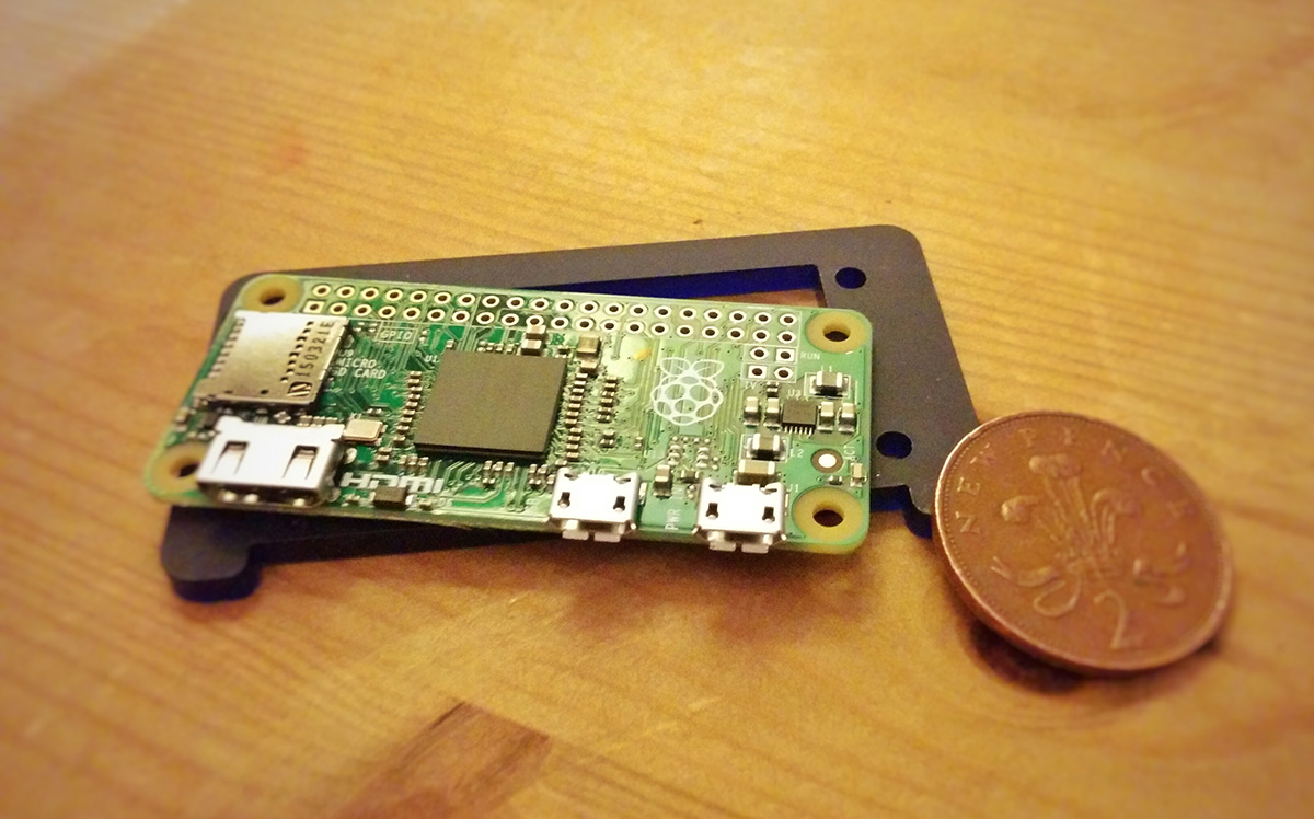
I will use a Raspberry Pi Zero because it is even cheaper and smaller than the normal Raspberry Pis, and the challenge to get a neural network running is even more worthy! It costs about £4 UK pounds, or $5 US dollars. That wasn’t a typo!

Here’s mine.

rasppi_zero.jpeg


Installing IPython

We’ll assume you have a Raspberry Pi powered up and a keyboard, mouse, display and access to the internet working.

There are several options for an operating system, but we’ll stick with the most popular which is the officially supported Raspian, a version of the popular Debian Linux distribution designed to work well with Raspberry Pis. Your Raspberry Pi probably came with it already installed. If not install it using the instructions at that link. You can even buy an SD card with it already installed, if you’re not confident about installing operating systems.

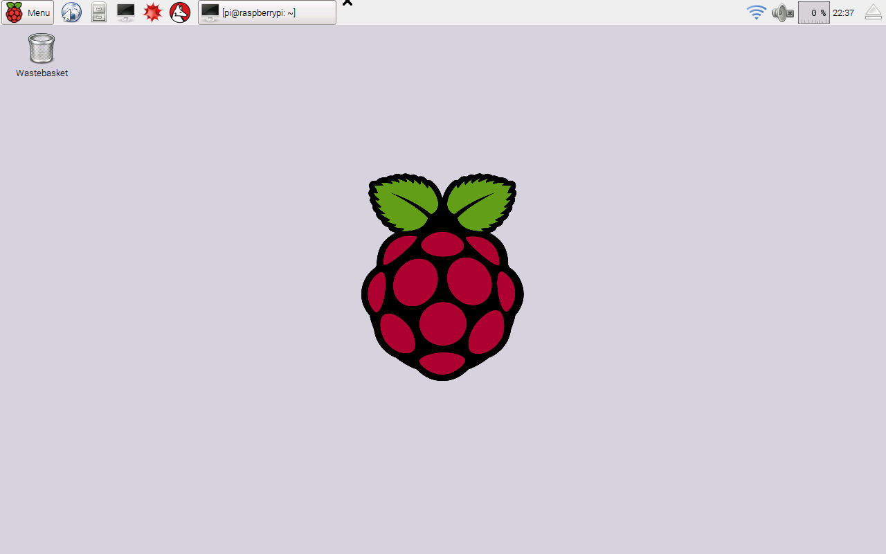
This is the desktop you should see when you start up your Raspberry Pi.

rasppi_0.png

You can see the menu button clearly at the top left, and some shortcuts along the top too.

We’re going to install IPython so we can work with the more friendly notebooks through a web browser, and not have to worry about source code files and command lines.

To get IPython we do need to work with the command line, but it’ll be just once, and the recipe is really simple and easy.

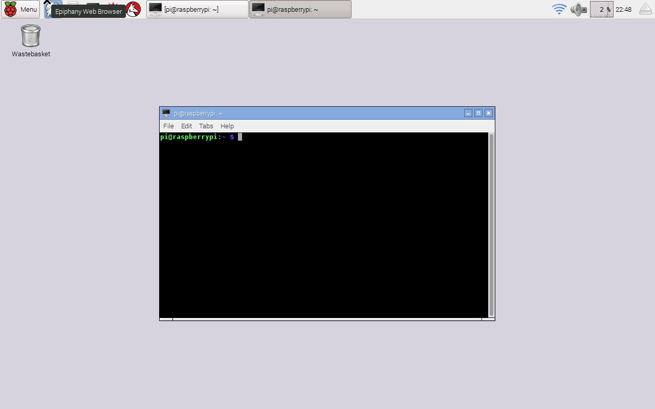
Open the Terminal application, which is the icon shortcut at the top which looks like a black monitor. If you hover over it, it’ll tell you it is the Terminal. When you run it, you’ll be presented with a black box, into which you type commands, looking like the this.

rasppi_1.png

Your Raspberry Pi is very good because it won’t allow normal users to issue commands that make deep changes. You have to assume special privileges. Type the following into the terminal:

sudo su -

You should see the prompt end in with a ‘#’ hash character. It was previously a ‘$’ dollar sign. That shows you now have special privileges and you should be a little careful what you type.

The following commands refreshes your Raspberry’s list of current software, and then updates the ones you’ve got installed, pulling in any new software if it’s needed.

apt-get upgrade
apt-get update

Unless you did this recently, there will likely be software that needs to be updated. You’ll see quite a lot of text fly by. You can safely ignore it. You may be prompted to confirm the update by pressing “y”.

Now that our Raspberry is all fresh and up to date, issue the command to get IPython. Note that, at the time of writing, the Raspian software packages don’t contain a sufficiently recent version of IPython to work with the notebooks we created earlier and put on github for anyone to view and download. If they did, we would simply issue a simple “apt-get install ipython3 ipython3-notebook” or something like that.

If you don’t want to run those notebooks from github, you can happily use the slightly older IPython and notebook versions that come from Raspberry Pi’s software repository.

If we do want to run more recent IPython and notebook software, we need to use some “pip” commands in additional to the “apt-get” to get more recent software from the Python Package Index. The difference is that the software is managed by Python (pip), not by your operating system’s software manager (apt). The following commands should get everything you need.

apt-get install python3-matplotlib
apt-get install python3-scipy

pip3 install ipython
pip3 install jupyter
pip3 install matplotlib
pip3 install scipy

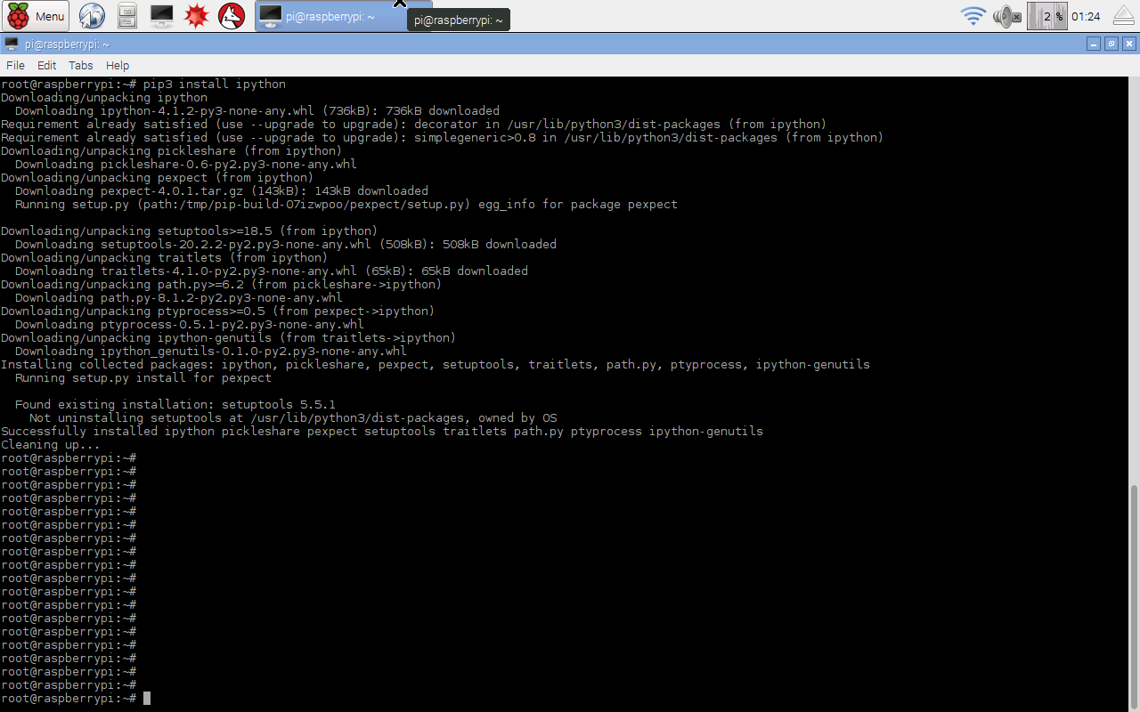
After a bit  of text flying by, the job will be done. The speed will depend on your particular Raspberry Pi model, and your internet connection. The following shows my screen when I did this.

rasppi_2.png

The Raspberry Pi normally uses an memory card, called an SD card, just like the ones you might use in your digital camera. They don’t have as much space as a normal computer. Issue the following command to clean up the software packages that were downloaded in order to update your Raspberry Pi.

apt-get clean

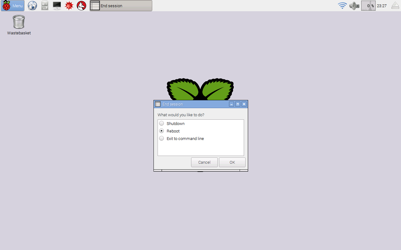
That’s it, job done. Restart your Raspberry Pi in case there was a particularly deep change such as a change to the very core of your Raspberry Pi, like a kernel update. You can restart your Raspberry Pi by selecting the “Shutdown …” option from the main menu at the top left, and then choosing “Reboot”, as shown next.

rasppi_3.png

After your Raspberry Pi has started up again, start IPython by issuing the following command from the Terminal:

jupyter notebook

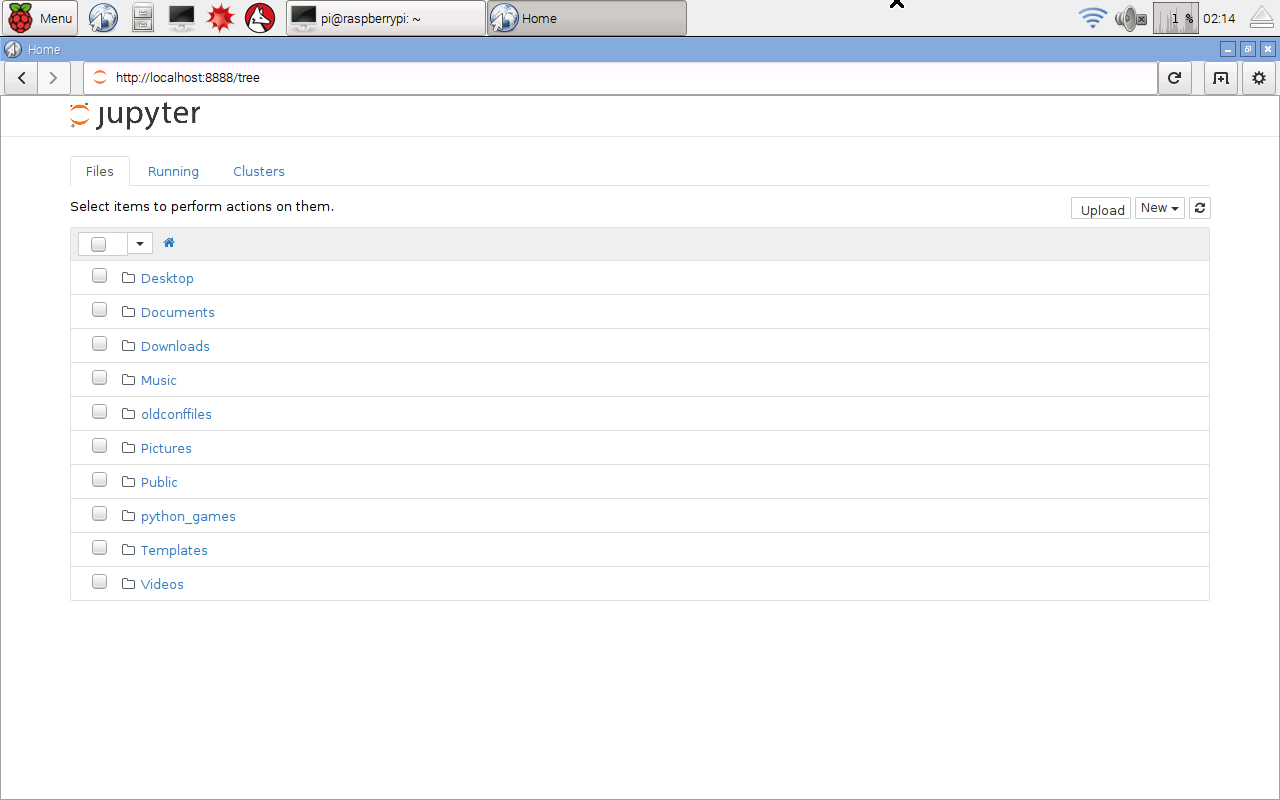
This will automatically launch a web browser with the usual IPython main page, from where you can create new IPython notebooks. Jupyter is the new software for running notebooks. Previously you would have used the “ipython3 notebook” command, which will continue to work for a transition period. The following shows the main IPython starting page.

rasppi_4.png

That’s great! So we’ve got IPython up and running on a Raspberry Pi.

You could proceed as normal and create your own IPython notebooks, but we’ll demonstrate that the code we developed in this guide does run. We’ll get the notebooks and also the MNIST dataset of handwritten numbers from github. In a new browser tab go to the link:


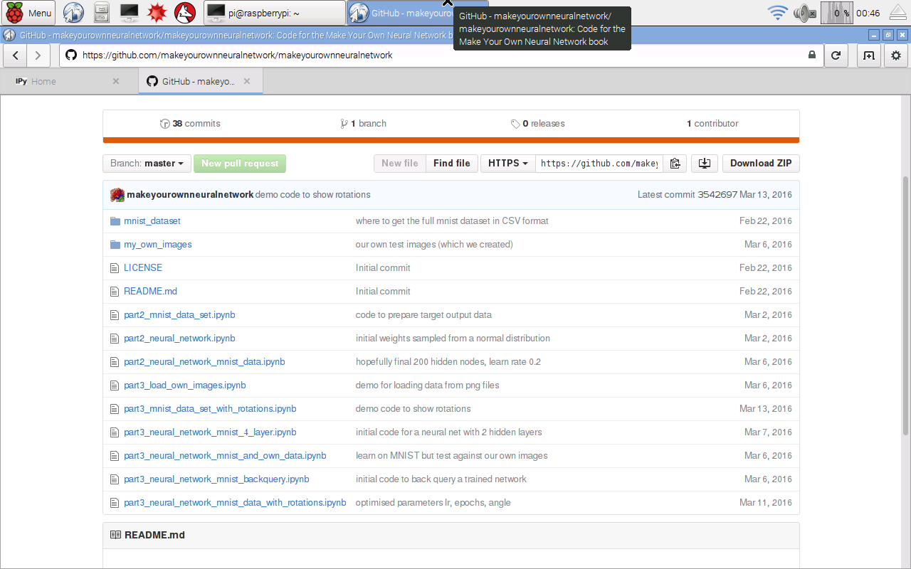
You’ll see the github project page, as shown next. Get the files by clicking “Download ZIP” at the top right.

rasppi_5.png

The browser will tell you when the download has finished. Open up a new Terminal and issue the following command to unpack the files, and then delete the zip package to clear space.

unzip Downloads/makeyourownneuralnetwork-master.zip
rm -f Downloads/makeyourownneuralnetwork-master.zip

The files will be unpacked into a directory called makeyourownneuralnetwork-master. Feel free to rename it to a shorter name if you like, but it isn’t necessary.

The github site only contains the smaller versions of the MNIST data, because the site won’t allow very large files to be hosted there. To get the full set, issue the following commands in that same terminal to navigate to the mnis_dataset directory and then get the full training and test datasets in CSV format.

cd makeyourownneuralnetwork-master/mnist_dataset

The downloading may take some time depending on your internet connection, and the specific model of your Raspberry Pi.

You’ve now got all the IPython notebooks and MNIST data you need. Close the terminal, but not the other one that launched IPython.

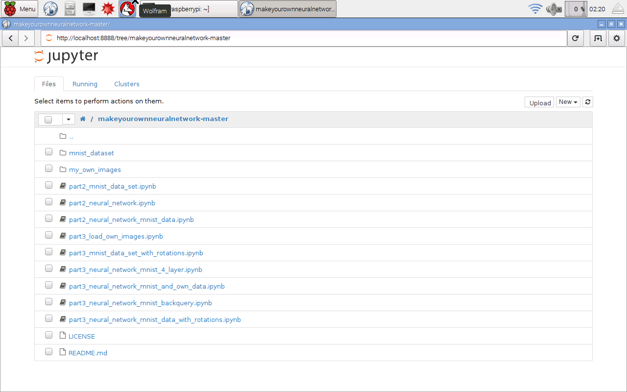
Go back to the web browser with the IPython starting page, and you’ll now see the new folder makeyourownneuralnetwork-master showing on the list. Click on it to go inside. You should be able to open any of the notebooks just as you would on any other computer. The following shows the notebooks in that folder.

rasppi_6.png


Making Sure Things Work

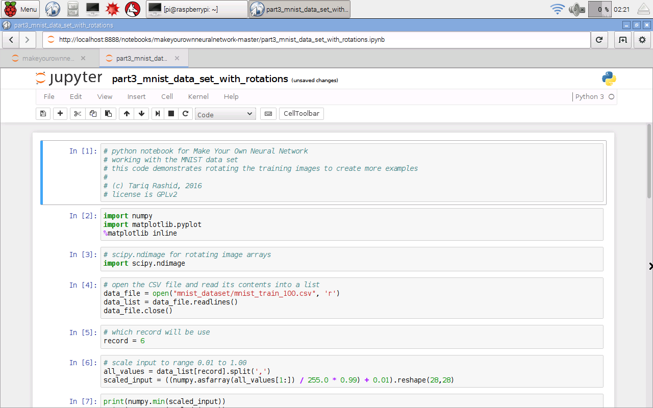
Before we train and test a neural network, let’s first check that the various bits, like reading files and displaying images, are working. Let’s open the notebook called “part3_mnist_data_set_with_rotations.ipynb” which does these tasks. You should see the notebook open and ready to run as follows.

rasppi_7.png

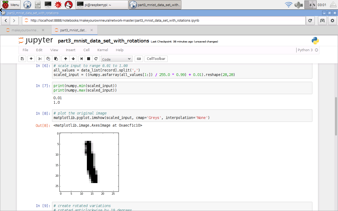
From the “Cell” menu select “Run All” to run all the instructions in the notebook. After a while, and it will take longer than a laptop, you should get some images of rotated numbers.

rasppi_8.png

That shows several things worked, including loading the data from a file, importing the python extension modules for working with arrays and images, and plotting graphics.

Let’s now “Close and Halt” that notebook from the File menu. You should close notebooks this way, rather than simply closing the browser tab.


Training And Testing A Neural Network

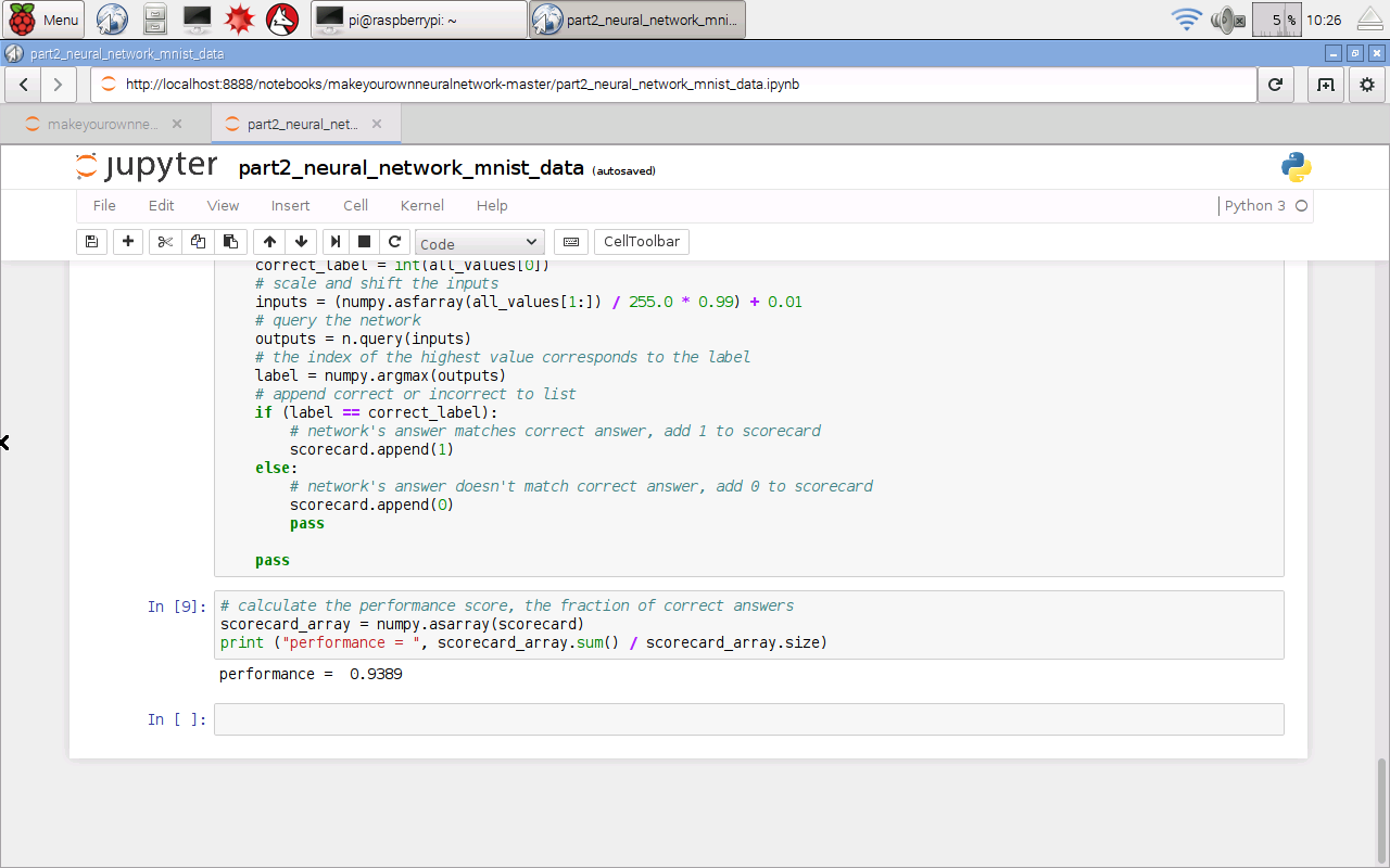
Now lets try training a neural network. Open the notebook called “part2_neural_network_mnist_data”. That’s  the version of our program that is fairly basic and doesn’t do anything fancy like rotating images. Because our Raspberry Pi is much slower than a typical laptop, we’ll turn down some of parameters to reduce the amount of calculations needed, so that we can be sure the code works without wasting hours and finding that it doesn’t.

I’ve reduced the number of hidden nodes to 50, and the number of epochs to 1. I still used the full MNIST training and test datasets, not the smaller subsets we created earlier. Set it running with “Run All” from the “Cell” menu. And then we wait ...

Normally this would take about one minute on my laptop, but this completed in about 25 minutes. That's not too slow at all, considering this Raspberry Pi Zero costs 400 times less than my laptop. I was expecting it to take all night.

rasppi_9.png


Raspberry Pi Success!

We’ve just proven that even with a £4 or $5 Raspberry Pi, you can still work fully with IPython notebooks and create code to train and test neural networks - it just runs a little slower!

Saturday 12 March 2016

Improving Neural Network Performance to 98% Accuracy!

The neural network we've developed is simple.

It has only one hidden layer. The activation function is simple. The process is straightforward. We've not done anything particularly fancy - though there are techniques and optimisations to boost performance.

And yet we've managed to get really good performance.

Yann LeCun is a world leading researcher and pioneer of neural networks - and his page lists some benchmarks for performance against the MNIST data set.


Let's go through the performance improvements that we can do without spoiling the simplicity that we've managed to retain on our journey:


94.7%

Our basic code had a performance of almost 95% is good for a network that we wrote at home, as begginers. It compares with the benchmarks on LeCun's website. A score of 60% or 30% would have been not so good but understandable as a first effort. Even a score of 85% would have been a solid starting point.


95.3%

We tweaked the learning rate and the performance broke through the 95% barrier. Keep in mind that there will be diminishing returns as we keep pushing for more performance. This is because there will be inherent limits - the data itself might have gaps or a bias, and so not be fully educational. The architecture of the network itself will impose a limit - architecture means the number of layers, the number of nodes in each layer, the activation function, the design of the labelling system, etc

The following shows the results of an experiment tweaking the learning rate. The shape of the performance curve is as expected - extremes away from a sweet spot give poorer performance.

Too low a learning rate and there isn't enough time (steps) to find a good solution by gradient descent. You may only have got halfway down the hill, as it were. Too high and you bounce around and overshoot the valleys in the error function landscape.


96.3%

Another easy improvement is running through the training data multiple times, called epochs. Doing it twice, instead of once, boosted the performance to 95.8%. Getting closer to that elusive 96%!

The following shows the results of trying different numbers of epochs.


You can see again there is a sweet spot around 5 epochs. I've left that odd dip in the graph, and not re-run the experiment for that data point for a good reason - to remind us that:
  • neural network learning is at heart a random process, and results will be different evert time, and sometimes will go wrong altogether
  • these experiments are not very scientific, to do that we'd have to run them many many times to reduce the impact of the randomness

The peak now is 96.3% with 7 epochs.


96.9%

Increasing the epochs means doing more traingin steps. Perhaps we can shorten the learning steps so that we are more cautious and reduce the chance of overshooting, now that we make up for smaller steps with more steps overall?

The following shows the previous experiment's results overlaid by the results with a smaller learning rate of 0.1.


There is a really good peak at 5 epochs with performance now boosted to 96.9%. That's very very good. And all without any really fancy tricks. We're getting closer to breaching the 97% mark!


97.6%

One parameter we haven't yet tweaked is the number of hidden nodes. This is an important layer because it is the one at the heart of any learning the network does. The input nodes simply bring in the question. The output nodes pretty much pop out the answer. It is the hidden nodes - or more strictly, the link weights either side of those nodes - that contain any knowledge the network has gained through learning.

Too few and there just usn't enough learning capacity. Too many and you dilute the learning and increase the time it takes to get to an effective learned state. Have a look at the following experiment varying the number of hidden nodes.


This is really interesting. Why? because even with 5 hidden nodes, a tiny number if you think about it, the performance is still amazing at 70%. That really is remarkable. The ability to do a complex task like recognise human handwritten numbers has been encoded by 5 nodes well enough to perform with 70% accuracy. Not bad at all.

As the number of nodes increases, the performance does too, but the returns are diminishing. The previous 100 nodes gives us 96.7% accuracy. Increasing the hidden layer to 200 nodes boosts the performance to 97.5%. We've broken the 97% barrier!

Actually, 500 hidden nodes gives us 97.6% accuracy, a small improvement, but at the cost of a much larger number of calculations and time taken to do them. So for me, 200 is the sweet spot.

Can we do more?


97.9% (!!!!)

We can do more, and the next idea is only mildly more sophisticated than our simple refinements above.

Take each training image, and create two new versions of each one byt rotating the original clockwise and anti-clockwise by a specific angle. This gives us new training examples, but ones which might add additional knowledge because they represent the possibility of somone writing those numbers are a different angle. The following illustrates this.


We've not cheated by taking new training data. We've used the existsng training data to create additional versions.

Let's see what performance we get if we run experiments with different angles. We've added in the results for 10 epochs just to see what happens too.


The peak for 5 epochs at +/- 10 degrees rotation is 97.5%.

Increase the epochs to 10 and we boost the performance to a record breaking 97.9% !!


This 2% error compares with amongst the best benchmarks. And all from simple ideas and simple code.


Isn't computer science cool ?!

Wednesday 9 March 2016

Inside the Mind of a Neural Network

Neural Network's Knowledge

Neural networks learn to solve problems in ways that are not entirely clear to us. The reason we use neural networks is that some problems are not easily reducible to simple solutions made up of a few short crisp rules. They're able to solve problems where we don't really know how to approach those problems, or what the key factors are in deciding what the answer should be.

In this sense, the "knowledge" that a neural network gains during training is somewhat mysterious and largely not understandable to us - the "mind" of a neural network.

Is there any way of seeing what this "mind" has become? It would be like seeing the dreams or hallucinations of a neural mind.


Backwards Query

Here's a crazy idea.

Normally we feed a question to a neural network's input nodes to see what the answer is popping out of the output nodes.

Why not feed answers into the output nodes - to see what questions pop out of the input nodes?
 

Since our network learns to recognise images of handwritten numbers - we can interpret the stuff that pops out of the input nodes as an image too, and hopefully an interesting image.

If we put signals that represent the label "5" into the output nodes, and get an image out of the input nodes, it makes sense that that the image is an insight into what the mind of the neural network thinks of "5".

Let's try it! The code to do this is on github:


The code is really simple:
  • We just propagate the signals backwards, using the link weights to moderate the signals as usual. Remember, these weights have already been refined through previous training - that is, the network has already "learned". 
  • The inverse of the logistic sigmoid is used when the signal goes backwards across a node, and it happens to be called a logit function.
  • There is an extra step where we rescale the signals at a layer before we use the logit function because they must be between 0 and 1 (not including 0 and 1). That is, logit(x) does not exist for x<=0 and x>=1.

The Label "0"

If we back query with the label "0" we get the following image popping out of the input nodes:


Well - that's interesting!

We have here a privileged insight into the mind of a neural network. As we'll see next, this is an insight into what and how it thinks.

How do we interpret this image?

  • Well it is round, which makes sense because we are asking it what the ideal question image would be to get a perfect output signal for the label "0".
  • There are light and dark and grey bits. 
  • The dark bits show which parts of the input image, if marked by handwriting, strongly indicate the answer would be a "0".
  • The light bits show which parts of the input image definitely need to be clear of any handwriting marks to indicate the answer would be a "0".
  • The grey bits are indifferent.

So we have actually understood what the neural network has learned about classifying images as "0".


More Brain-Scans

Let's have a look at the images that emerge from back-querying the rest of the digits (click to enlarge)


Wow - again some really interesting images.

They're like ultrasound scans into the brain of the neural network.

Some notes about these images:

  • The "7" is really clear. You can see the dark bits which, if marked in the query image, strongly suggest a a label "7". You can also see the additional "white" area which must be clear of any marking. Together these two characteristics indicate a "7".
  • Same applies to the "3" - there area areas which, if marked, indicate a "3", and areas which must be clear too. The "5" is similarly apparent too.
  • The "4" is interesting in that there is a shape which appears to have 4 quadrants, and excluded areas too. 
  • The "8" is largely made up of white areas suggesting that an eight is characterised by markings kept out of the central regions.

Some of the images are very clear and definite but some aren't and this might suggest that there is more learning to be done. Without more learning, the confidence in the network answering with the label "8" woud be lower than for a really clear "0", "5" or a "7".

Having said that, the network performs really really well anyway  - at 97.5% accuracy over the test set of 10,000 images!

So there you have it - a brain scan into the mind of a neural network!

Sunday 6 March 2016

Your Own Handwriting - The Real Test

We've trained and tested the simple 3 layer neural network on the MNIST training and test data sets. That's fine and worked incredibly well - achieving 97.4% accuracy!

The code in python notebook form is at github:
That's all fine but it would feel much more real if we got the neural network to work on our own handwriting, or images we created.

The following shows six sample images I created:


The 4 and 5 are my own handwriting using different "pens". The 2 is a traditional textbook or newspaper two but blurred. The 3 is my own handwriting but with bits deliberately taken out to create gaps. The first 6 is a blurry and wobbly character, almost like a reflectioni n water. The last 6 is the previous but with a layer of random noise added.

We've created deliberately challening images for our network. Does it work?

The demonstration code to train against the MNIST data set but test against 28x28 PNG versions of these images is at:
It works! The following shows a correct result for the damaged 3.


In fact the code works for all the test images except the very noisy one. Yippeee!


Neural Networks Work Well Despite Damage - Just Like Human Brains
There is a serious point behind that broken 3. It shows that neural networks, like biological brains, can work quite well even with some damage. Biological brains work well when damaged themselves, here the damage is to the input data, which is analogous. You could do your own experiments to see how well a network performs when random trained neurons are removed.