Wednesday 27 January 2016

Why a Squared Error Cost Function?

Why is the squared error most often used for training neural networks?
I must have read dozens of tutorials and papers, tens of slides and presentations, and a handful of proper academic textbooks too. And none of them seemed to explain well why the squared error function is used, and most read as if there could be no other choice.

This blog explores this question, poses a "naive" alternative derived from first principles, and demonstrates that it seems to work.


Basics

Let's recall some basics.
  • Neural networks are trained by adjusting the link weights.
  • The key factor that informs these adjustments is how "wrong" the untrained network is.
  • The actual output and the desired output (training examples) will be different in an untrained network.
  • This difference (target - actual) is the error. There is an error for each output layer node.


Cost Function

During network training, the weights are adjusted guided by a cost function. A cost function is a way of expressing how good or bad a neural network is. The shape of a cost function guides how weights need to change to improve the network's performance.

Intuitively, you can see that the cost function must be in some way related to the error above. 

Most guides will use the following cost function to minimise

$$Cost=\sum_{output\_nodes}(target−actual)^2$$

They often don't give a solid clear reason for this function, but if they do say anything it is the following:
    • the $(target - actual)^2$ is always positive so errors of different signs don't cancel out, potentially misrepresenting how "wrong" the network is. For example, errors of +2 and -2 from output nodes would sum to zero, suggesting a perfectly correct output where it is in fact clear the output nodes are in error. 
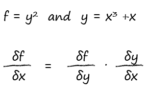
    • the cost function is differentiable so we can work out the sensitivity of the error to individual weights, the partial differential $$\frac{\partial {Cost}}{\partial {w}}$$
    • parallels to linear regression, where errors are assumed to be Gaussian, that is, distributed normally around the true value.


Challenge

I challenge each of the above points in turn:

  • We don't need the cost function to always be positive because we don't actually sum over the errors from each output node. Instead we consider each output node in turn and in isolation from any other output node when we propagate the errors back.
  • You can find $\frac{\partial {Error}}{\partial {w}}$ from the simpler naive $Error=(target−actual)$. There is no problem deriving the partial differentials from this $Error$ expression. Instead of trying to minimise it, we instead move towards zero from either direction. We're trying towards zero $Error$, not to get it to ever lower values below zero.
  • There is no reason to believe the errors in the output of a neural network are distributed normally.


Weight Learning from a Naive Cost Function

The following are the steps for deriving a weight update expression from a simpler naive cost function that isn't the squared error function.

  • Consider only one output node of a neural network, the $jth$ node.
  • The error at the $jth$ output node is $(target - actual)$, or $e_j=(t_j−o_j)$.
  • The actual output, $o_j=sigmoid(\sum{w_i.x_i})$ where $w_i$ is the weight of the $ith$ link to that $jth$ node, and $x_i$ is the output from the preceding $ith$ node. The $sigmoid(x)$ is the popular squashing function $\frac{1}{(1+e^{−x})}$.
  • So $$\frac{\partial {e_j}}{\partial {w_k}} = \frac{\partial}{\partial{w_k}}(t_j - o_j) =  \frac{\partial}{\partial{w_k}}(- sigmoid(\sum_{i}w_i.x_i))$$ because we can ignore the constant $t_j$. We can also see that only one $w_{i=k}$ matters as other $w_{i≠k}$ don't contribute to the differential. That simplifies the sum inside the sigmoid.
  • That leaves us with $$\frac{\partial {e_j}}{\partial {w_k}} =  \frac{\partial}{\partial{w_k}}(- sigmoid(w_k.x_k)) = −(w_k.x_k)(1−w_k.x_k).x_k$$ because we know how to differentiate the sigmoid.
So we have an expression for $\frac{\partial {e_j}}{\partial {w_k}}$ which can be used to guide the iterative refinement of the weight $w_k$ so that $e_j$ moves towards zero from both directions.

From both directions? Let's unfold that a bit more.

If the error at a node $e_j=(t_j−o_j)$ is positive, and the gradient with respect to weight $w_k$ is positive, we reduce the weight. If the gradient is negative, we increase the weight. In this way we inch towards zero error.

The opposite applies if the error is negative. If the gradient is positive we increase the weight a bit, and if it is negative, we decrease the weight a bit.

The following diagram illustrates this gradient ascent or descent towards zero from both directions, and compares it with the descent only using the squared error cost function.


We've only derived the weight update expression for the link weights between the hidden and output layer of a node. The logic to extend this to previous layers is no different to normal neural network backpropagation - the errors are split backwards across links in proportion to the link weight, and recombined at each hidden layer node. This is illustrated as follows with example numbers:


Does It Work? ... Yes!!

I coded the necessary changes into the existing neural network python code, and the results compare really favourably.

Here's the Python notebook for a neural network learning to classify the MNIST image data set using the normal squared error cost function. The basic unoptimised code achieves 97% accuracy on the 10,000 test set.

Python Notebook - gradient descent to minimise squared error. 97% success.

Now here's the same Python notebook but altered to to gradient ascent and descent aiming to zero the naive cost function.

Python Notebook - gradient ascent and descent to zero naive error. 93% success.

The size of this accuracy at 93% over the 10,000 test data instances from the MNIST set means this isn't a lucky fluke. This works.

My next thoughts are ... what are the advantages of this grad ascent/descent?
  • Do we lose some information by the act of squaring? Because we've lost the +ve and -ve aspects?
  • Should we stick to the squared error because the actual accuracy was slightly higher when compared like for like?
  • Why are the actual output values much better polarised towards the extremes of zero and one using this naive function? With learning rate 0.3 the test of item 20 in the test set results in a stark output histogram.


Did I Go Wrong?

For me this challenges the unquestioning acceptance of the squared error cost function.

But I might be very very mistaken. Do get in touch on twitter @myoneuralnet


Update

Thanks to help from the London Kaggle Meetup the following is now clear to me:

  • The naive error function has a gradient that is linear, and trying to optimise it by moving towards zero is the same as trying to move to the bottom zero of the absolute value error $|target-outout|$. 
  • The refinements are not as efficient as the size of the step is constant - which risks bouncing about the minimum or the zero. 
  • You could mitigate this by moderating the step size in proportion to the closeness to the target. This means multiplying the step change by the error $(target-output)$. This in effect is the same calculation as that from the squared error cost function!
This is the second time the London Kaggle Meetup has helped me get through a barrier!

Tuesday 12 January 2016

A Gentle Introduction to Calculus

This post is taken from a draft Appendix to the upcoming Make Your Own Neural Network. It aims to introduce the idea of calculus and differentiation in a gentle manner, sufficient to understand the backpropagation algorithm used to train neural networks.

I'd love feedback on how successful this draft is in helping as many people as possible understand calculus.


Imagine you’re in a car cruising smoothly and relaxed at a constant 30 miles per hour. Imagine you then press the accelerator pedal. If you keep it pressed your speed increases to 35, 40, 50, and 60 miles per hour.

The speed of the car changes.

In this section we’ll explore the idea of things changing - like the speed of a car - and how to work out that change mathematically. What do we mean, mathematically? We mean understanding how things are related to each other, so we can work out precisely how  changes in one result in changes in another. Like car speed changing with the time on my watch. Or plant height changing with rain levels. Or the extension of a metal spring changing as we apply different amounts of pulling force.

This is called calculus by mathematicians. I hesitated about calling this section calculus because many people seem to think that is a hard scary subject to be avoided. That’s a real shame, and the fault of bad teaching and terrible school textbooks.

By the end of this appendix, you’ll see that working out how things change in a mathematically precise way - because that’s all calculus is really - is not that difficult for many useful scenarios.

Even if you’ve done calculus or differentiation already, perhaps at school, it is worth going through this section because we will understand how calculus was invented back in history. The ideas and tools used by those pioneering mathematicians are really useful to have in your back pocket, and can be very helpful when trying to solve different kinds of problems in future.

If you enjoy a good historical punch-up, look up the drama between Leibnitz and Newton who both claimed to have invested calculus first!


A Flat Line

Let’s first start with a very easy scenario to get ourselves settled and ready to go.

Imagine that car again, but cruising at a constant speed of 30 miles per hour. No faster, not slower, just 30 miles per hour.

Here’s a table showing the speed at various points in time, measured every half a minute.

Time (mins)
Speed (mph)
0.0
30
0.5
30
1.0
30
1.5
30
2.0
30
2.5
30
3.0
30

The following graph visualises this speed at those several points in time.


You can see that the speed doesn’t change over time, that’s why it is a straight horizontal line. It doesn’t go up (faster) or down (slower), it just stays at 30 miles per hour.

The mathematical expression for the speed, which we call s, is

Now, if someone asked how the speed changes with time, we’d say it didn’t. The rate of change is zero. In other words, the speed doesn’t depend on time. That dependency is zero.

We’ve just done calculus! We have, really!

Calculus is about establishing how things change as a result of other things changing. Here we are thinking about how speed changes with time.

There is a mathematical way of writing this.

What are those symbols? Think of the symbols meaning “how speed changes when time changes”, or “how does s depend on t”.

So that expression is a mathematician’s concise way of saying the speed doesn’t change with time. Or put another way, the passing of time doesn’t affect speed. The dependency of speed on time is zero. That’s what the zero in the expression means. They are completely independent. Ok, ok - we get it!

In fact you can see this independence when you look again at the expression for the speed, s = 30. There is no mention of the time in there at all. That is, there is no symbol t hidden in that expression. So we don’t need to do any fancy calculus to work out that ∂s / ∂t = 0, we can do it by simply looking at the expression. Mathematicians call this “by inspection”.

Expressions like ∂s / ∂t, which explain a rate of change, are called derivatives. We don’t  need to know this for our purposes, but you may come across that word elsewhere.

Now let’s see what happens if we press the accelerator. Exciting!


A Sloped Straight Line

Imagine that same car going at 30 miles per hour. We press the accelerator gently and the car speeds up. We keep it pressed and watch the speed dial on the dashboard and note the speed every 30 seconds.

After 30 seconds the car is going at 35 miles per hour. After 1 minute the car is now going at 40 miles per hour. After 90 it’s going at 45 miles per hour, and after 2 minutes it’s 50 miles per hour. The car keeps speeding up by 10 miles per hour every minute.

Here’s the same information summarised in a table.

Time (mins)
Speed (mph)
0.0
30
0.5
35
1.0
40
1.5
45
2.0
50
2.5
55
3.0
60

Let’s visualise this again.


You can see that the speed increases from 30 miles per hour all the way up to 60 miles per hour at a constant rate. You can see this is a constant rate because the increments in speed are the same every half a minute and this leads to a straight line for speed.

What’s the expression for the speed? Well we must have speed 30 at time zero. And after that we add an extra 10 miles per hour every minute. So the expression is as follows.

Or using symbols,
You can see the constant 30 in there. And you can also see the (10 * time) which adds the 10 miles per hour for every minute. You’ll quickly realise that the 10 is the gradient of that line we plotted. Remember the general form of straight lines is y = ax + b where a is the slope, or gradient.

So what’s the expression for how speed changes with time? Well, we’ve already been talking about it, speed increases 10 mph every minute.

What this is saying, is that there is indeed a dependency between speed and time. This is because ∂s / ∂t is not zero.

Remembering that the slope of a straight line y = ax+b is a, we can see “by inspection” that the slope of s = 30+10t will be 10.

Great work! We’ve covered a lot of the basics of calculus already, and it wasn’t that hard at all.

Now let’s hit that accelerator harder!


A Curved Line

Imagine I started the car from stationary and hit the accelerator hard and kept it pressed hard. Clearly the starting speed is zero because we’re not moving initially.

Imagine we’re pressing the accelerator so hard that the car doesn’t increase it’s speed at a constant rate. Instead it increases it’s speed in faster way. That means, it is not adding 10 miles per hour every minute. Instead it is adding speed at a rate that itself goes up the longer we keep that accelerator pressed.

For this example, let’s imagine the speed is measured every minute as shown in this table.

Time (mins)
Speed (mph)
0
0
1
1
2
4
3
9
4
16
5
25
6
36
7
49
8
64

If you look closely you might have spotted that I’ve chosen to have the speed as the square of the time in minutes. That is, the speed at time 2 is 22=4, and at time 3 is 32=9, and time 4 is 42=16, and so on.

The expression for this is easy to write too.
Yes, I know this is a very contrived example of car speed, but it will illustrate how we might do calculus really well.

Let’s visualise this so we can get a feel for how the speed changes with time.


You can see the speed zooming upwards at an ever faster rate. The graph isn’t a straight line now. You can imagine that the speed would explode to very high numbers quite quickly. At 20 minutes the speed would be 400 miles per hour. And at 100 minutes the speed would be 10,000 miles per hour!

The interesting question is - what’s the rate of change for the speed with respect to time?

This isn’t the same as asking, what is the actual speed at a particular time. We already know that because we have the expression s = t2.

What we’re asking is this - at any point in time, what is the rate of change of speed? Not what is the speed. What does this even mean?

If we think back to our previous two examples, we saw that the rate of change was the slope of the graph of speed against time. When the car was cruising at a constant 30, the speed wasn’t changing, so it’s rate of change was zero. When the car was getting faster steadily, it’s rate of change was 10 miles per hour every minute. And that 10 mph every minute was true for any point in time. At time 2 minutes the rate of change was 10 mph/min. And it was true at 4 minutes and would be true at 100 minutes too.

Can we apply this same thinking to this curved graph? Yes we can - but let’s go extra slowly here.


Calculus By Hand

Let’s look more closely at what is happening at time 3 minutes.

At 3 minutes, the speed is 9 miles per hour. We know it will be faster after 3 minutes. Let’s compare that with what is happening at 6 minutes. At 6 minutes, the speed is 36 miles per hour. We also know that the speed will be faster after 6 minutes.

But we also know that a moment after 6 minutes the speed increase will be greater than an equivalent moment after 3 minutes. There is a real difference between what’s happening at time 3 minutes and time 6 minutes.

Let’s visualise this as follows.


You can see that the slope at time 6 minutes is steeper than at time 3 minutes. These slopes are the rate of change we want. This is an important realisation, so let’s say it again. The rate of change of a curve at any point, is the slope of the curve at that point.

But how do we measure the slope of a line that is curved? Straight lines were trivial, but curvy lines? We could try to estimate the slope by drawing a straight line, called a tangent, which just touches that curved line in a way that tries to be at the same gradient as the curve just at the point. This is in fact how people used to do it before other ways were invented.

Let’s try rough and ready method, just so we have some sympathy with that approach. The following diagram shows the speed graph with a tangent touching the speed curve at time 6 minutes.


To work out the slope, or gradient, we know from school maths that we need to divide the height of the incline by the extent. In the diagram this height (speed) is shown as Δs, and the extent (time) is shown as Δt. That symbol, Δ called “delta”, just means a small change. So Δt is a small change in t.

The slope is Δs / Δt. We could chose any sized triangle for the incline, and use a ruler to measure the height and extent. With my measurements I just happen to have a triangle with Δs measured as 9.6, and Δt as 0.8. That gives the slope as follows:


We have a key result! The rate of change of speed at time 6 minutes is 12.0 mph per min.

You can see that relying on a ruler, and even trying to place a tangent by hand, isn’t going to be very accurate. So let’s let’s get a tiny bit more sophisticated.

Calculus Not By Hand

Look at the following graph which has a new line marked on it. It isn’t the tangent because it doesn’t touch the curve only at a single point. But is does seem to be centred around time 3 minutes in some way.


In fact there is connection to time 3 minutes. What we’ve done is chosen a time above and below this point of interest at t=3. Here, we’ve selected points 2 minutes above and below t=3 minutes. That is, t=1 and t=5 minutes.

Using our mathematical notation, we say we have a Δx of 2 minutes. And we have chosen points x-Δx and x+Δx. Remember that symbol Δ just means a “small change”, so Δx is a small change in x.

Why have we done this? It’ll become clear very soon - hang in there just a bit.

If we look at the speeds at times x-Δx and x+Δx, and draw a line between between those two points, we have something that very roughly has the same slope as a tangent at the middle point x. Have a look again at the diagram above to see that straight line. Sure, it’s not going to have exactly the same slope as a true tangent at x,  but we’ll fix this.

Let’s work out the gradient of this line. We use the same approach as before where the gradient is the height of the incline divided by the extent. The following diagram makes clearer what the height and extent is.


The height is the difference between the two speeds at  x-Δx and  x+Δx, that is, 1 and 5 minutes. We know the speeds are 1 and 25 mph at these points so the difference is 24. The extent is the very simple distance between  x-Δx and  x+Δx, that is, between 1 and 5, which is 4. So we have:


The gradient of the line, which is approximates the tangent at t=3 minutes, is 6 mph per min.

Let’s pause and have a think about what we’ve done. We first tried to work out the slope of a curved line by hand drawing a tangent. This approach will never be accurate, and we can’t do it many many times because, being human, we’ll get tired, bored, and make mistakes. The next approach doesn’t need us to hand draw a tangent, instead we follow a recipe to create a different line which seems to have approximately the right slope. This second approach can be automated by a computer and done many times and very quickly, as no human effort is needed.

That’s good but not good enough yet!

That second approach is only an approximation. How can we improve it so it’s not an approximation? That’s our aim after all, to be able to work out how things change, the gradient, in a mathematically precise way.

This is where the magic happens! We’ll see one of the neat tools that mathematicians have developed and kept largely for themselves!

What would happen if we made the extent smaller? Another way of saying that is, what would happen if we made the Δx smaller? The following diagram illustrates several approximations or slope lines resulting from a decreasing Δx.


We’ve drawn the lines for Δx = 2.0, Δx = 1.0, Δx = 0.5 and Δx = 0.1. You can see that the lines are getting closer to the point of interest at 3 minutes. You can imagine that as we keep making Δx smaller and smaller, the line gets closer and closer to a true tangent at 3 minutes.

As Δx becomes infinitely small, the line becomes infinitely closer to the true tangent. That’s pretty cool!

This idea of approximating a solution and improving it by making the deviations smaller and smaller is very powerful. It allows mathematicians to solve problems which are hard to attack directly. It’s a bit like creeping up to a solution from the side, instead of running at it head on!


Calculus without Plotting Graphs

We said earlier, calculus is about understanding how things change in a mathematically precise way. Let’s see if we can do that by applying this idea of ever smaller Δx to the mathematical expressions that define these things - things like our car speed curves.

To recap, the speed is a function of the time that we know to be s = t2. We want to know how the speed changes as a function of time. We’ve seen that is the slope of s when it is plotted against t.

This rate of change ∂s / ∂t is the height divided by the extent of our constructed lines but where the Δx gets infinitely small.

What is the height? It is (t + Δx)2 - (t - Δx)2 as we saw before. This is just s=t2 where t is a bit below and a bit above the point of interest. That amount of bit is Δx.

What is the extent? As we saw before, it is simply the distance between (t+Δx) and (t-Δx) which is 2Δx.

We’re almost there,


Let’s expand and simplify that expression,


We’ve actually been very lucky here because the algebra simplified itself very neatly.

So we’ve done it! The mathematically precise rate of change is ∂s / ∂t = 2t. That means for any time t, we know the rate of change of speed ∂s / ∂t = 2t.

At t=3 minutes we have ∂s / ∂t = 2t = 6. We actually confirmed that before using the approximate method. For t=6 minutes, ∂s / ∂t = 2t = 12, which nicely matches what we found before too.

What about t = 100 minutes? ∂s / ∂t = 2t = 200 mph per minute. That means after 100 minutes, the car is speeding up at a rate of 200 mph per minute.

Let’s take a moment to ponder the magnitude and coolness of what we just did. We have a mathematical expression that allows us to precisely know the rate of change of the car speed at any time. And following our earlier discussion, we can see that changes in s do indeed depend on time.

We were lucky that the algebra simplified nicely, but the simple s=t2 didn’t give us an opportunity to try reducing the Δx in an intentional way. So let’s try another example where the speed of the car is only just a bit more complicated,


What is the height now? It is the difference between s calculated at t+Δx and s calculated at t-Δx. That is, the height is (t + Δx)2 + 2(t +Δx ) - (t - Δx)2 - 2(t -Δx).

What about the extent? It is simply the distance between (t+Δx) and (t-Δx) which is still 2Δx.


Let’s expand and simplify that expression,


That’s a great result! Sadly the algebra again simplified a little too easily. It wasn’t wasted effort because there is a pattern emerging here which we’ll come back to.

Let’s try a another example, which isn’t that much more complicated. Let’s set the speed of the car to be the cube of the time.


Let’s expand and simplify that expression,


Now this is much more interesting! We have a result which contains a Δx, whereas before they were all cancelled out.

Well, remember that the gradient is only correct as the Δx gets smaller and smaller, infinitely small.

This is the cool bit! What happens to the expression ∂s / ∂t = 3t2 + Δx2 as Δx gets smaller and smaller? It disappears! If that sounds surprising, think of a very small value for Δx. If you try, you can think of an even smaller one. And an even smaller one .. and you could keep going forever, getting ever closer to zero. So let’s just get straight to zero and avoid all that hassle.

That gives is the mathematically precise answer we were looking for:


That’s a fantastic result, and this time we used a powerful mathematical tool to do calculus, and it wasn’t that hard at all.


Patterns

As fun as it is to work out derivatives using deltas like Δx and seeing what happens when we make them smaller and smaller, we can often do it without doing all that work.

See if you can see any pattern in the derivatives we’ve worked out so far:


You can see that the derivative of a function of t is the same function but with each power of t reduced by one. So t4 becomes t3, and t7 would become t6, and so on. That’s really easy! And if you remember that t is just t1, then in the derivative it becomes t0, which is 1.

Constants numbers on their own like 3 or 4 or 5 simply disappear. Constant variables on their own, which we might call a, b or c, also disappear, because they too have no rate of change. That’s why they’re called constants.

But hang on, t2 became 2t no just t. And t3 became 3t2 not just t2. Well there is an extra step where the power is used as a multiplier before it is reduced. So the 5 in 2t5 is used as an additional multiplier before the power is reduced 5*2t4 = 10t4.

The following summarises this power rule for doing calculus.


Let’s try it on some more examples just to practice this new technique.


So this rule allows us to do quite a lot of calculus and for many purposes it’s all the calculus we need. Yes, it only works for polynomials, that is expressions made of variables with powers like y = ax3 + bx2 + cx +d, and not with things like sin(x) or cos(x). That’s not a major flaw because there are a huge number of uses for doing calculus with this power rule.

However for neural networks we do need one extra power, which we’ll look at next.


Functions of Functions

Imagine a function
where y is itself
We can write this as f = (x3+x)2 if we wanted to.

How does f change with y? That is, what is ∂f / ∂y ? This is easy as we just apply the power rule we just developed, multiplying and reducing the power, so ∂f / ∂y = 2y.

What about a more interesting question. How does f change with x? Well we could expand out the expression f = (x3+x)2 and apply this same approach. We can’t can’t apply it naively to (x3+x)2 to become 2(x3+x).

If we worked many of these out the long hard way, using the diminishing deltas approach like before, we’d stumble upon another set of patterns. Let’s jump straight to the answer.

The pattern is this:


This is a very powerful result, and is called the chain rule.

You can see that it allows us to work out derivatives in layers, like onion rings, unpacking each layer of complexity. To work out ∂f / ∂x we might find it easier to work out ∂f / ∂y and then also easier to work out ∂y / ∂x. If these are easier, we can then do calculus on expressions that otherwise look quite impossible. The chain rule allows us to break a problem into smaller easier ones.

Let’s look at that example again and apply this chain rule:


We now work out the easier bits. The first bit is ( ∂f / ∂y ) = 2y. The second bit is ( ∂y / ∂x ) = 3x2 +1. So recombining these bits using the chain rule we get

We know that y = x3+x so we can have an expression with only x


Magic!

You may challenge this as ask why we didn’t just expand out f in terms of x first and then apply simple power rule calculus to the resulting polynomial. We could have done that, but we wouldn’t have illustrated the chain rule, which allows us to crack much harder problems.

Let’s look at just one final example because it shows us how to handle variables which are independent of other variables.

If we have a function
where x, y and z are independent of each other. What do we mean by independent? We mean that x, y and z can be any value and don’t care what the other variables are - they aren’t affected by changes in the other variables. This wasn’t the case in previous example where y was x3 + x, so y was dependent on x.

What is ∂f / ∂x? Let’s look at each part of that long expression. The first bit is 2xy, so the derivative is 2y. Why is this so simple? It’s because y is not dependent on x. What we’re asking when we say ∂f / ∂x is how does f change when x changes. If x doesn’t depend on y, we can ignore it because doesn’t affect f. It might as well be another number like 2 or 3 or 10.

Let’s carry on. The next bit is 3x2z. We can apply the power reduction rule to get 2*3xz or 6xz. We treat z as just a boring number like 2 or 4 or maybe 100, because x is independent of z. A change in z doesn’t affect x.

The final bit 4z has no x in it at all. So it vanishes, because we treat it like a plain constant number like 2 or 4.

The final answer is
The important thing in this last example is having the confidence to ignore variables that you know are independent. It makes doing calculus on quite complex expressions drastically simpler, and it is an insight we’ll need lots when looking at neural networks.


You can do Calculus!

If you got this far, well done!

You have a genuine insight into what calculus really is, and how it was invented using approximations that get better and better. You can always try these methods on other tough problems that resist normal ways for solving them.

The two techniques we learned, reducing powers and the chain rule, allows us to do quite a lot of calculus, including understanding how neural networks really work and why.

Enjoy your new powers!