Saturday 14 March 2020

Thursday 5 March 2020

Gradient Descent Unstable For GANs?

When training neural networks we use gradient descent to find a path down a loss function to find the combination of learnable parameters that minimise the error. This is a very well researched area and techniques today are very sophisticated, the Adam optimiser being a good example.

The dynamics of a GAN are different to a simple neural network. The generator and discriminator networks are trying to achieve opposing objectives. There are parallels between a GAN and adversarial games where one player is trying to maximise an objective while the other is trying to minimise it, each undoing the benefit of the opponent’s previous move.

Is the gradient descent method of finding the correct, or even good enough, combination of learnable parameters suitable for such adversarial games? This might seem like an unnecessary question, but the answer is rather interesting.


Simple Adversarial Example


The following is a very simple objective function:


One player has control over the values of x and is trying to maximise the objective f. A second player has control over y and is trying to minimise the objective f.

Let’s visualise this function to get a feel for it. The following picture shows a surface plot of f = x·y from three slightly different angles.


We can see that the surface of f = x·y is a saddle. That means, along one direction the values rise then fall, but in another direction, the values fall then rise.

The following picture shows the same function from above, using colours to indicate the values of f. Also marked are the directions of increasing gradient.


If we used our intuition to find a good solution to this adversarial game, we would probably say the best answer is the middle of that saddle at (x,y) = (0,0). At this point, if one player sets x = 0, the second player can’t affect the the value of f no matter what value of y is chosen. The same applies if y = 0, no value of x can change the value of f. The actual value of f at this point is also the best compromise. Elsewhere there are as many higher values of f as there are lower, so it seems like a good compromise.

You can explore the surface interactively yourself using the math3d.org website:


Let’s now move away from intuition and work out the answer by simulating both players using gradient descent, each trying to find a good solution for themselves.

You’ll remember from Make Your Own Neural Network that parameters are adjusted by a small amount that depends on the gradient of the objective function.


The reason we have different signs in these update rules is that y is trying to minimise f by moving down the gradient, but x is trying to maximise f by moving up the gradient. That lr is the usual learning rate.

Because we know f = x·y we can write those update rules with the gradients worked out.


We can write some code to pick starting values for x and y, and then repeatedly apply these update rules to get successive x and y values.

The following shows how x and y evolve as training progresses.


We can see that the values of x and y don’t converge, but oscillate with ever greater amplitude. Trying different starting values leads to the same behaviour. Reducing the learning rate merely delays the inevitable divergence.

This is bad. It shows that gradient descent can’t find a good solution to this simple adversarial game, and even worse, the method leads to disastrous divergence.

The following picture shows x and y plotted together. We can see the values orbit around the ideal point (0,0) but run away from it.


It can be shown mathematically (see below) that the best case scenario is that (x,y) orbits in a fixed circle around the (0,0) without getting closer to it, but this is only when the update step is infinitesimally small. As soon we have a finite step size, as we do when approximate that continuous process in discrete steps, the orbit diverges.

You can explore the code which plays this adversarial game using gradient descent here:


Gradient Descent Isn’t Ideal For Adversarial Games


We’ve shown that gradient descent fails to find a solution to an adversarial game with a very simple objective function. In fact, it doesn’t just fail to find a solution, it catastrophically diverges. In contrast, gradient descent used in the normal way to minimise a function is guaranteed to find a minimum, even if it isn’t the global minimum.

Does this mean GAN training will fail in general? No.

Realistic GANs with meaningful data will have much more complex loss functions, and that can reduce the chances of runaway divergence. That’s why GAN training throughout this book has worked fairly well. But this analysis does indicate why training GANs is hard, and can become chaotic. Orbiting around a good solution might also explain why some GANs seem to progress onto different modes of single-mode collapse with extended training rather than improving the quality of images themselves.

Fundamentally, gradient descent is the wrong approach for GANs, even if it works well enough in many cases. Finding optimisation techniques designed for adversarial dynamics like those in GANs is currently an open research question, with some researchers already publishing encouraging results.


Why A Circular Orbit?


Above we stated that (x,y) orbits as a circle when two players each use gradient descent to optimise f = x·y in opposite directions. Here we’ll do the maths to show why it is a circle.

Let’s look at the update rules again.


If we want to know how x and y evolve over time t, we can write:


If we take the second derivatives with respect to t, we get the following.


You may remember from school algebra that expressions of the form d2y/dt2 = - a2x have a solution the form y = sin(at) or y = cos(at). To satisfy the first derivatives above, we need x and y to be the following combination.


These describe (x,y) moving around a unit circle with angular speed lr.

Monday 17 February 2020

Calculating the Output Size of Convolutions and Transpose Convolutions

Convolution is common in neural networks which work with images, either as classifiers or as generators. When designing such convolutional neural networks, the shape of data emerging from each convolution layer needs to be worked out.

Here we’ll see how this can be done step-by-step with configurations of convolution that we’re likely to see working with images.

In particular, transposed convolutions are thought of as difficult to grasp. Here we’ll show that they’re not difficult at all by working though some examples which all follow a very simple recipe.


Example 1: Convolution With Stride 1, No Padding


In this first simple example we apply a 2 by 2 kernel to an input of size 6 by 6, with stride 1.


The picture shows how the kernel moves along the image in steps of size 1. The areas covered by the kernel do overlap but this is not a problem. Across the top of the image, the kernel can take 5 positions, which is why the output is 5 wide. Down the image, the kernel can also take 5 positions, which is why the output is a 5 by 5 square. Easy!

The PyTorch function for this convolution is:

nn.Conv2d(in_channels, out_channels, kernel_size=2, stride=1)


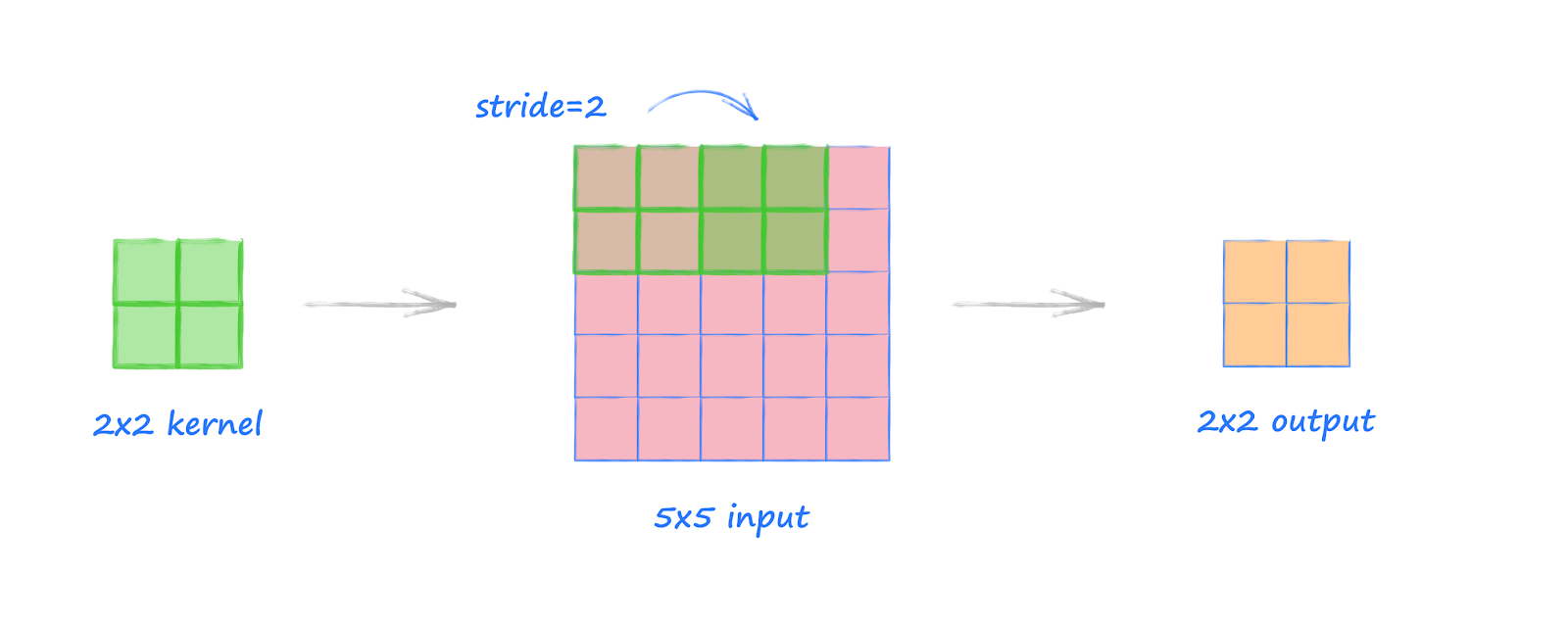
Example 2: Convolution With Stride 2, No Padding


This second example is the same as the previous one, but we now have a stride of 2.


We can see the kernel moves along the image in steps of size 2. This time the areas covered by the kernel don’t overlap. In fact, because the kernel size is the same as the stride, the image is covered without overlaps or gaps. The kernel can take 3 positions across and down  the image, so the output is 3 by 3.

The PyTorch function for this convolution is:

nn.Conv2d(in_channels, out_channels, kernel_size=2, stride=2)


Example 3: Convolution With Stride 2, With Padding


This third example is the same as the previous one, but this time we use a padding of 1.


By setting padding to 1, we extend all the image edges by 1 pixel, with values set to 0. That means the image width has grown by 2. We apply the kernel to this extended image. The picture shows the kernel can take 4 positions across the image. This is why the output is 4 by 4.

The PyTorch function for this convolution is:

nn.Conv2d(in_channels, out_channels, kernel_size=2, stride=2, padding=2)


Example 4: Convolution With Coverage Gaps


This example illustrates the case where the chosen kernel size and stride mean it doesn’t reach the end of the image.


Here, the 2 by 2 kernel moves with a step size of 2 over the 5 by 5 image. The last column of the image is not covered by the kernel.

The easiest thing to do is to just ignore the uncovered column, and this is in fact the approach taken by many implementations, including PyTorch. That’s why the output is 2 by 2.

For medium to large images, the loss of information from the very edge of the image is rarely a problem as the meaningful content is usually in the middle of the image. Even if it wasn’t, the fraction of information lost is very small.

If we really wanted to avoid any information being lost, we’d adjust some of the option. We could add a padding to ensure no part of the input image was missed, or we could adjust the kernel and stride sizes so they matches the image size.


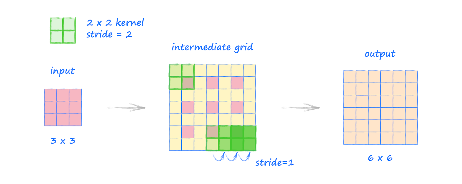
Example 5: Transpose Convolution With Stride 2, No Padding


The transpose convolution is commonly used to expand a tensor to a larger tensor. This is the opposite of a normal convolution which is used to reduce a tensor to a smaller tensor.

In this example we use a 2 by 2 kernel again, set to stride 2, applied to a 3 by 3 input.


The process for transposed convolution has a few extra steps but is not complicated.

First we create an intermediate grid which has the original input’s cells spaced apart with a step size set to the stride. In the picture above, we can see the pink cells spaced apart with a step size of 2. The new in-between cells have value 0.

Next we extend the edges of the intermediate image with additional cells with value 0. We add the maximum amount of these so that a kernel in the top left covers one of the original cells. This is shown in the picture at the top left of the intermediate grid. If we added another ring of cells, the kernel would no longer cover the original pink cell.

Finally, the kernel is moved across this intermediate grid in step sizes of 1. This step size is always 1. The stride option is used to set how far apart the original cells are in the intermediate grid. Unlike normal convolution, here the stride is not used to decide how the kernel moves.

The kernel moving across this 7 by 7 intermediate grid gives us an output of 6 by 6.

Notice how this transformation of a 3 by 3 input to a 6 by 6 output is the opposite of Example 2 which transformed an input of size 6 by 6 to an output of size 3 by 3, using the same kernel size and stride options.

The PyTorch function for this transpose convolution is:

nn.ConvTranspose2d(in_channels, out_channels, kernel_size=2, stride=2)


Example 6: Transpose Convolution With Stride 1, No Padding


In the previous example we used a stride of 2 because it is easier to see how it is used in the process. In this example we use a stride of 1.


The process is exactly the same. Because the stride is 1, the original cells are spaced apart without a gap in the intermediate grid. We then grow the intermediate grid with the maximum number of additional outer rings so that a kernel in the top left can still cover one of the original cells. We then move the kernel with step size 1 over this intermediate 7 by 7 grid to give an output of size 6 by 6.

You’ll notice this is the opposite transformation to Example 1.

The PyTorch function for this transpose convolution is:

nn.ConvTranspose2d(in_channels, out_channels, kernel_size=2, stride=1)


Example 7: Transpose Convolution With Stride 2, With Padding


In this transpose convolution example we introduce padding. Unlike the normal convolution where padding is used to expand the image, here it is used to reduce it.

We have a 2 by 2 kernel with stride set to 2, and an input of size 3 by 3, and we have set padding to 1.


We create the intermediate grid just as we did in Example 5. The original cells are spaced 2 apart, and the grid is expanded so that the kernel can cover one of the original values.

The padding is set to 1, so we remove 1 ring from around the grid. This leaves the grid at size 5 by 5. Applying the kernel to this grid gives us an output of size 4 by 4.

The PyTorch function for this transpose convolution is:

nn.ConvTranspose2d(in_channels, out_channels, kernel_size=2, stride=2, padding=1)


Calculating Output Sizes


Assuming we’re working with square shaped input, with equal width and height, the formula for calculating the output size for a convolution is:


The L-shaped brackets take the mathematical floor of the value inside them. That means the largest integer below or equal to the given value. For example, the floor of 2.3 is 2.

If we use this formula for Example 3, we have input size = 6, padding = 1, kernel size = 2. The calculation inside the floor brackets is (6 + 2 - 1 -1) /2 + 1, which is 4. The floor of 4 remains 4, which is the size of the output.

Again, assuming square shaped tensors, the formula for transposed convolution is:


Let’s try this with Example 7, where the input size = 3, stride = 2, padding = 1, kernel size = 2. The calculation is then simply 2*2 - 2 + 1 + 1 = 4, so the output is of size 4.

On the PyTorch references pages you can read about more general formulae, which can work with rectangular tensors and also additional configuration options we’ve not needed here.


More Reading


Wednesday 12 September 2018

Application of Neural Networks - Satellite Measurement of Water Waves

It's always great to see interesting uses of machine learning methods - and especially satisfying to see someone inspired by my book to apply the methods.

I was privileged to have an initial discussion with Dennis when he was planning on applying neural networks to the task of classifying water waveforms measured by radar from a satellite orbiting the Earth.

He went on to succeed and presented his work at a well respected conference. You can see his presentation slides here:


Altimetry

Satellite radar is used to measure the altitude (height) of surface features - which can be both land and water.


The signal needs to be interpreted and so that:

  • we can establish if the surface is land or water
  • and if water, calculate the height of the water waves from the non-trivial signal pattern


Land or Water?

A neural network was trained to determine whether the signal was from land or water.


As you can see from the slide above, the signal signature is very different.

A neural network was very successful in detecting water. Detecting land was a little more challenging but this initial work showed great promise.


Water Wave Height

The next step is to calculate the height of the water waves. In-situ measurements were used as reference data to train a different neural network.

Part of the challenge for a neural network is that there are several peaks that can be detected during a measurement, and we want the highest peak of a wave.


Tracking a peak as it moves allows us to have a higher level of confidence in labelling it a water wave peak.


Results

The results are promising with some areas identified for further work.

The following shows how good the calculated water wave heights are based on automatic analysis by neural networks.


The first area for improvement is detecting land where the accuracy rate is lower than it is for water.

The second area for further work is to the resolve the "delay" visible in the calculated heights. This is not a major issue in this application as the height and shape are more important than the horizontal displacement / phase.

The following shows more challenging wave forms.


A good next challenge is to automate the detection of the correct peak, and neural network architectures that take into account a sequence of data - such as recurrent neural networks - can help in these scenarios.


Tuesday 22 May 2018

Imageio.imread() Replaces Scipy.misc.imread()

Some of the code we wrote reads data from image files using a helper function scipy.misc.imread().

However, recently, users were notified that this function is deprecated:


We're encouraged to use the imageio.imread() function instead.

From imread() to imread()

The change is very easy. We first change the import statements which include the helper library.

From this:
import scipy.misc

To this:
import imageio

We then change the actual function which reads image data from files.

From this form:
img_array = scipy.misc.imread(image_file_name, flatten=True)

To this form:
img_array = imageio.imread(image_file_name, as_gray=True)

Easy!

We can see the new function is used in a very similar way. We still provide the name of the image file we want to read into a array of data.

Previously we used flattern=True to convert the image pixels into a greyscale value, instead of having separate numbers for the red, green, blue and maybe alpha channels. We now use as_grey=True which does the same thing.

I thought we might have to mess about with inverting number ranges from 0-255 to 255-0 but it seems we don't need to.


Github Code Updated

The notebooks which use imread() have been updated on the main github repository.

This does mean the code is slightly different to that described in the book, but the change should be easy to understand until a new version of the book is released.

Wednesday 16 May 2018

Online Interactive Course by Educative.io

I've been really impressed with educative.io who took the content for Make Your Own Neural Network and developed a beautifully designed interactive online course.


The course breaks the content down into digestible bite-size chunks, and the interactivity is really helpful to the process of learning through hands-on experimentation and play.

Have a go!


Wednesday 7 February 2018

Saving and Loading Neural Networks

A very common question I get is how to save a neural network, and load it again later.


Why Save and Load?

There are two key scenarios when being able to save and load a neural network are useful.

  • During a long training period it is sometimes useful to stop and continue at a later time. This might be because you're using a laptop which can't remain on all the time. It could be because you want to stop the training and test how well the neural network performs. Being able to resume training at a different time is really helpful.
  • It is useful to share your trained neural network with others. Being able to save it, and for someone else to load it, is necessary for this to work.


What Do We Save?

In a neural network the thing that is doing the learning are the link weights. In our Python code, these are represented by matrices like wih and who. The wih matrix contains the weights for the links between the input and hidden layer, and the who matrix contains the weights for the links between the hidden and output layer.

If we save these matrices to a file, we can load them again later. That way we don't need to restart the training from the beginning.


Saving Numpy Arrays

The matrices wih and who are numpy arrays. Luckily the numpy library provides convenience functions for saving and load them.

The function to save a numpy array is numpy.save(filename, array). This will store array in filename. If we wanted to add a method to our neuralNetwork class, we could do it simply it like this:

# save neural network weights 
def save(self):
    numpy.save('saved_wih.npy', self.wih)
    numpy.save('saved_who.npy', self.who)
    pass

This will save the wih matrix as a file saved_wih.npy, and the wih matrix as a file saved_wih.npy.

If we want to stop the training we can issue n.save() in a notebook cell. We can then close down the notebook or even shut down the computer if we need to.


Loading Numpy Arrays

To load a numpy array we use array = numpy.load(filename). If we want to add a method to our neuralNetwork class, we should use the filenames we used to save the data.

# load neural network weights 
def load(self):
    self.wih = numpy.load('saved_wih.npy')
    self.who = numpy.load('saved_who.npy')
    pass

If we come back to our training, we need to run the notebook up to the point just before training. That   means running the Python code that sets up the neural network class, and sets the various parameters like the number of input nodes, the data source filenames, etc.

We can then issue n.load() in a notebook cell to load the previously saved neural networks weights back into the neural network object n.


Gotchas

We've kept the approach simple here, in line with our approach to learning about and coding simple neural networks. That means there are some things our very simple network saving and loading code doesn't do.

Our simple code only saves and loads the two wih and who weights matrices. It doesn't do anything else. It doesn't check that the loaded data matches the desired size of neural network. We need to make sure that if we load a saved neural network, we continue to use it with the same parameters. For example, we can't train a network, pause, and continue with different settings for the number of nodes in each layer.

If we want to share our neural network, they need to also be running the same Python code. The data we're passing them isn't rich enough to be independent of any particular neural network code. Efforts to develop such an open inter-operable data standard have started, for example the Open Neural Network Exchange Format.


HDF5 for Very Large Data

In some cases, with very large networks, the amount of data to be saved and loaded can be quite big. In my own experience from around 2016, the normal saving of bumpy arrays in this was didn't always work. I then fell back to a slightly more involved method to save and load data using the very mature HDF5 data format , popular in science and engineering.

The Anaconda Python distribution allows you to install the h5py package, which gives Python the ability to work with HDF5 data.

HDF5 data stores do more than the simple data saving and loading. They have the idea of a group or folder which can contain several data sets, such as numpy arrays. The data stores also keep account of data set names, and don't just blindly save data. For very large data sets, the data can be traverse and segmented on-disk without having to load it all into memory before subsets are taken.

You can explore more here: http://docs.h5py.org/en/latest/quick.html#quick